The quality of the data while training an intelligent model is one of the most important parameters that affect the performance of the model directly. It is believed that low-volume, high-quality data is better than high volume pooer quality data, simply meaning “Garbage In, Garbage Out’.

Multicollinearity is also one of the concepts in machine learning that one comes across while learning and working in the field of Artificial Intelligence and Data Science. It is very essential to have a thoro understanding of such terminologies, in order to deal with scenarios, where multicollinearity is encountered.

In this article, we will discuss the concept of multicollinearity, the core idea behind it, and its importance of the same. This article will help one to understand the concept of multicollinearity and will be able to make necessary changes and decisions to the data according to the same.

So let us now dive into that.

What is Multicollinearity?

Multicollieanrty in machine learning is a term used to describe the correlation among the dataset’s features. In machine learning, before applying an algorithm to the dataset, we have two types of features or columns, and those are the independent variables and dependent variables. Multicollinearity describes the correlation among the independent features of the dataset.

The data having correlations among the independent features of the dataset is known as multicolinear data and is also called the data with multicollinearity present. Here the correlated features or columns of the dataset change as per the values of other variables of feature changes on which the other variable is correlated.

For example, if we have weight and height as a feature of out dataset, then the correlation between these two features can be high normally, and hence, the multicollinearity is said to be present between these two variables.

Now let us discuss the techniques which are used to measure the multicollinearity in the dataset.

Variance Inflation Factor (VIF)

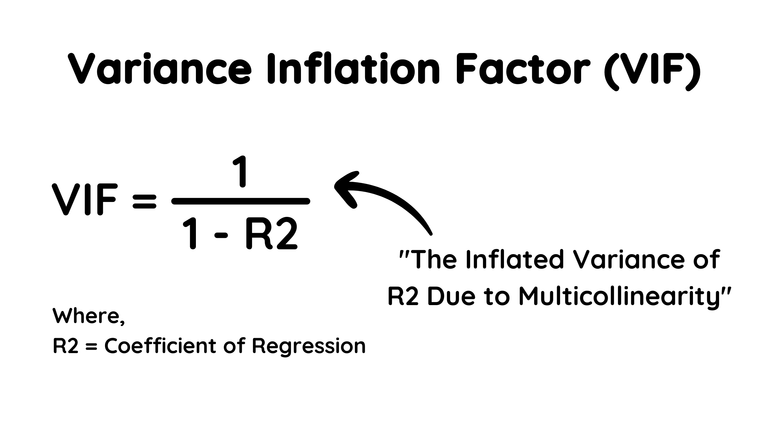
The variance inflation factor, or the VIF, is a measure of the multicollinearity of the independent variables of the dataset. It is a type of score that quantifies the multicollinearity for each independent variable in the dataset.

The formula for the VIF score is:

VIF = 1 / 1- R2

Where,

R2 = R squared score of the model.

The R2 score of the model is measured with the help of validating the model’s predictions on the test data or the unknown data. Higher the R2 score, the higher the performance of the model.

As the name suggests, the VIF score si the measure of the inflation of the variance of the R2 score of the model. In simple words, it is the measure of variance inflation of the R2 score due to multicollinearity.

The VIF score has an advantage over the correlation matrix, where it can be used to describe the effect of multicollinearity of different variables on the R2 score of the model.

Here the value of teh VIF score can vary for different variables, and mainly, three categories are defined for the same.

1. VIF = 1: In this case, the variable does not have any multicollinearity present.
2. VIF = 1 to 5: In this case, a small amount of multicollinearity is present in the dataset, but it is acceptable.
3. VIF > 5: In this case, the dataset is said to have very high multicollinearity, and operational steps should be taken to remove the same from the data.

Now a gentle question may appear in our mind if the VIF score signifies the multicollinearity or the correlation between the independent features, then the correlation matrix can also be used, then what is the need for a VIF score? Let us answer the question in the next section.

Correlation Matrix Vs. VIF Score

The concept of the VIF score and the correlation matrix is almost the same, where both of these measures the correlation between the features and tell us about the relationship of independent features of the dataset. However, there is a slight difference between them.

Correlation Matrix

In the case of the correlation matrix, it is a simple matrix that is a measure of the relationship between two variables of the dataset and tells us about the strength and direction of the relationship.

Its values lie between -1 to 1, where -1 means strong negative correlation, 0 means no correlation, and 1 means strong positive correlation.

Here note that we can check if the variables are related to each other and how strongly they are related, but with the help of correlation, we can not measure the effect of this relation on the model’s performance.

Variance Inflation factor (VIF)

The Variance inflation factor or the VIf score is also the measure of the relationship between different variables of the dataset, but it specifically tells us about the effect of these relationships of multicollinearity on the model’s performance as well. It can have values lying between 1 to 10 (In some cases, more than 10).

Here is the R2 score used in the formula of the VIF score; it tells us how the R2 score is inflated due to multicollinearity. So to measure the multicollinearity and its effect, the VUF score is a better choice than the correlation matrix.

Now let us discuss about the variance inflation factor code example and let us try to visualize the same.

Variance Inflation Factor: Example

Here to understand the multicollinearity and the variance inflation factor, we will use a dummy dataset with multicollinearity present.

Step 1: Generating the Dataset

Here we will generate a dummy dataset with 100 rows and 5 features with multicollinearity present in the dataset. Here the dataset will contain features name, height, weight, age, and gender.

import numpy as np

import pandas as pd

np.random.seed(42)

# Generate correlated variables

age = np.random.randint(18, 65, size=100)

weight = age + np.random.normal(0, 10, size=100)

height = age + np.random.normal(0, 5, size=100)

name = np.random.choice(['John', 'Mary', 'David', 'Sarah'], size=100)

gender = np.random.choice(['Male', 'Female'], size=100)

# Create a DataFrame

data = pd.DataFrame({'Age': age, 'Weight': weight, 'Height': height, 'Name': name, 'Gender': gender})

Step 2: Feature Engineering

Now we will convert the categorical variables in the numerical form to train the regression model on the same.

# Separate dependent and independent variables

X = data[['Age', 'Height']]

categorical_cols = ['Name', 'Gender']

# One-hot encode categorical variables

encoder = OneHotEncoder(drop='first', sparse=False)

encoded_cols = encoder.fit_transform(data[categorical_cols])

encoded_col_names = encoder.get_feature_names_out(categorical_cols)

encoded_cols_df = pd.DataFrame(encoded_cols, columns=encoded_col_names)

Step 3: Defining X and Y variables

Here the model’s task would be to predict the weight of the person, which is a regression problem.

# Concatenate numeric and encoded categorical variables

X = pd.concat([X, encoded_cols_df], axis=1)

y = data['Weight']

Step 4: Training the Linear regression Model

Now training the linear regression model with X and y training data. Here the R2 score of the model will help us get the VIF score of the dataset’s features.

# Fit a linear regression model

model = LinearRegression()

model.fit(X, y)

Step 5: Plotting the Correlation Matrix

Now let us plot the correlation matrix of the data. Here in default, we will plot the Pearson correlation matrix.

# Plot correlation matrix

plt.figure(figsize=(8, 6))

sns.heatmap(data.corr(), annot=True, cmap='coolwarm', linewidths=0.5)

plt.title('Correlation Matrix')

plt.show()

Output

Step 6: Calculating the VIF score of the Variables

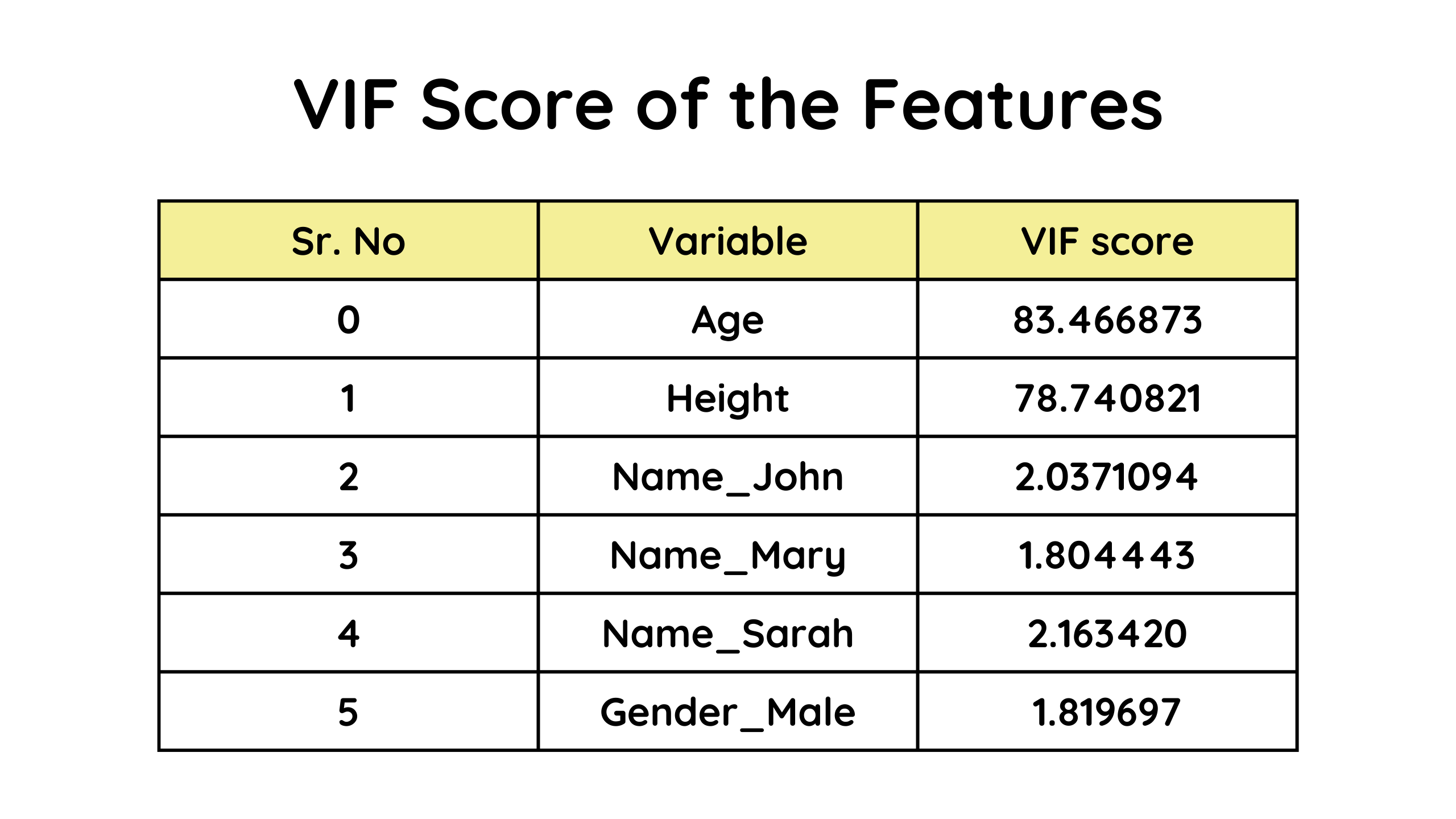
Now let us calculate the VIF score for all teh independent variables of the dataset. It will give us an idea about the multicollinearity present in the database and the effect of the same on the R2 score or the model’s performance.

# Calculate VIF scores

vif_data = pd.DataFrame()

vif_data['Variable'] = X.columns

vif_data['VIF'] = [variance_inflation_factor(X.values, i) for i in range(X.shape[1])]

# Display VIF scores

print('VIF Scores:')

print(vif_data)

Output

As we can clearly see that the height and the age columns have very high values of the VIF score, which directly means that they are highly correlated and have multicollinearity present. In such cases, either one of the features can be dropped or both the features can be combined into one.

Now let us discuss some of the ways we can deal with multicollinearity.

Ways to Deal With Multicollinearity

Once we have detected the multicollinearity, the very next task is to eliminate it from the dataset, as it can have a very bad impact on the performance of the model. There are some ways we can consider to deal with the multicollinearity present.

1. Drop Correlated Features

If the correlated features are very similar and have very less importance for the model, then dropping them is one of the easiest and fastest ways to deal with multicollinearity. However, the importance of features and model performance should be considered before that.

2. Use Dimensionality Reduction Techniques

If multicollinearity is present in the dataset, the dimensionality reduction techniques like PCA or t-SNE can be used to reduce the dimensions of the data. These techniques may eliminate the multicollinearity from the dataset.

3. Gather More Data

Although gathering a very high amount of data for each problem statement is not possible all the time, if possible, more and more data can be used to train the model in order to eliminate the multicollinearity.

4. Use Regularizations

Regularization methods like ridge or lasso regression can be used to deal with multicollinearity. Here these methods introduce the penalty term to the regression model and shrink the coefficient estimates to mitigate the multicollinearity of the dataset.

5. Feature Engineering

The features engineering can be used in order to deal with multicollinearity. Some of the correlated features can be combined together, some of them can be dropped, some of them can be scaled, some of them can be transformed, etc.

Key Takeaways

1. Multicollinearity is a term used when the features of the dataset are correlated among themselves.

2. The multilinearity can be harmful in the case of linear regression and naive bayes as they are parametric machine learning algorithms that assume the data to be free of multicollinearity.

3. The Variance inflation factor or the VIF score can be used in order to check for the multicollinearity present in the dataset.

4. VIF score is simply the measure of variance inflation of the R2 score of the model, which signified the effect of multicollinearity of the data on the R2 score or performance of the model.

5. We can drop the correlated features or apply dimensionality reduction techniques to the dataset to handle the multicollinearity in the dataset.

Conclusion

In this article, we discussed Multicollinearity, the core idea behind it, where it can damage the model, the idea behind the VIF score, what does it signified, how it is calculated, the difference between correlation and VIF score, the code example of the multicollinearity, and how it can be handled.

To conclude the multicollinearity is the correlation between the independent variables of the dataset and which be detected with the help of correlation matrics and VIF score. The VIF score sis a more robust way to detect multicollinearity in the dataset and which should be handled before deploying the model.

This article will help one to clear the concept of multicollinearity and VIF scores and will be able to apply and use the same concepts wherever necessary. It will also help one to answer interview questions related to the same.